Performing Simulations
The Pmetrics simulator is a powerful Monte Carlo engine that is smoothly integrated with Pmetrics inputs and outputs. Unlike NPAG and IT2B, it is run from within R. No batch file is created or terminal window opened. However, the actual simulator is a Fortran executable compiled and run in an OS shell.
To complete a simulator run you must include data and a model object.
These can be previously loaded objects with PM_data() and
PM_model() or loaded on the fly by specifying file names of
appropriate files in the current working directory, which you can check
with getwd() and list.files(), e.g., .csv for
data and .txt for models, at the time of simulation. The model dictates
the equations and the data file serves as the template specifying doses,
observation times, covariates, etc.
The other mandatory item is a prior probability distribution for all
random parameter values in the model. This is referenced by the
poppar argument, detailed below.
You run the simulator in two ways.
- Use the
$sim()method forPM_result()objects. This takespopparfrom thePM_result$finalfield and the model from thePM_result$modelfield, so only a data object needs to be specified at minimum. If no data object is specified, it will use thePM_result$dataas a template, i.e. the same data used to fit the model. An example is below. You don’t have to supply the model orpoppar, because they are included inrun1, withpoppartaken from therun$finalfield. Supplying a differentPM_dataobject asdatallows you to use the model and population prior fromrun1with a different dosing and observation data template. If you omitdatin this example, the original data inrun1would serve as the template.
run1 <- PM_load(1)
sim1 <- run1$sim(data = dat, nsim = 100, limits = NA)- Use
PM_sim$new(). This simulates without necessarily having completed a fitting run previously, i.e., there may be noPM_result()object. Here, you manually specify values forpoppar,model, anddata. These can be other Pmetrics objects, or de novo, which can be useful for simulating from models reported in the literature. An example is below.
sim2 <- PM_sim$new(poppar = run2$final, data = dat, model = mod1,...)Now you must include all three of the mandatory arguments:
model, data, and poppar. In this
case we used the PM_final() object from a different run
(run2) as the poppar, but we could also
specify poppar as a list, for example. See
SIMrun() for details on constructing a manual
poppar.
Under the hood, both of these calls to the simulator use the Legacy SIMrun() function, and thus
all its arguments are available when using
PM_result$sim(...) or PM_sim$new(...).
Model and data details
The structures of the model and data objects when used by the
simulator are identical to those used by NPAG and IT2B. Of course, the
model primary (random) parameters must match the parameters in the
poppar argument. Any covariates must match between model
and data. The data object contains the template dosing and observation
history as well as any covariates. Observation values (the
OUT column) for EVID=0 events can be any
number; they will be replaced with the simulated values. However, do not
use -99, as this will simulate a missing value, which might be useful if
you are testing the effects of such values. A good choice for the OUT
value in the simulator data template is -1 to remind you that it is
being simulated, but this choice is optional.
You can have any number of subject records within a data object, each
with its own covariate values if applicable. Each subject will cause the
simulator to run one time, generating as many simulated profiles as you
specify from each template subject. This is controlled by the
include, exclude, and nsim
arguments to the simulator (see below). The first two specify which
subjects in the data object will serve as templates for simulation. The
second specifies how many profiles are to be generated from each
included subject.
Simulation options
Details of all arguments available to modify simulations are
available by typing ?SIMrun into the R console or reading
the documentation for SIMrun(). A few are highlighted
here.
Simulation from a non-parametric prior distribution (from NPAG) can
be done in one of two ways. The first is simply to take the mean and
covariance matrix of the distribution and perform a standard Monte Carlo
simulation. This is accomplished by setting split = FALSE
as an argument.
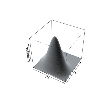
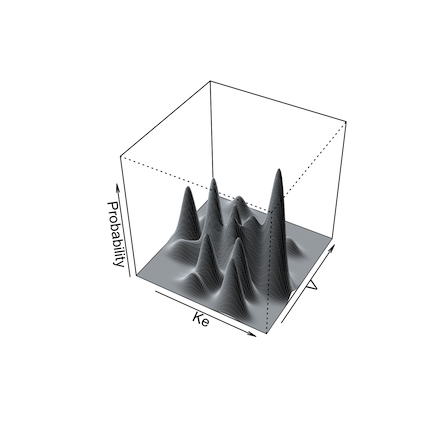
The second way is what we call semi-parametric (Goutelle et al. 2022). In this method, the non-parametric “support points” in the population model, each a vector of one value for each parameter in the model and the associated probability of that set of parameter values, serve as the mean of one multi-variate normal distribution in a multi-modal, multi-variate joint distribution. The weight of each multi-variate distribution is equal to the probability of the point. The overall population covariance matrix is divided by the number of support points and applied to each distribution for sampling.
Below are illustrations of simulations with a single mean and
covariance for two parameters (left, split = FALSE), and
with multi-modal sampling (right, split = TRUE).
Limits may be specified for truncated parameter ranges to avoid
extreme or inappropriately negative values. The simulator will report
values for the total number of simulated profiles needed to generate
nsim profiles within the specified limits, as well as the
means and standard deviations of the simulated parameters to check for
simulator accuracy.
Output from the simulator can be controlled by further arguments
passed to SIMrun(). If makecsv is supplied, a
.csv file with the simulated profiles will be created with the name as
specified by makecsv; otherwise, there will be no .csv file
created. If outname is supplied, the simulated values and
parameters will be saved in a .txt file whose name is that specified by
outname; otherwise the filename will be “simout”. In either
case, integers 1 to the number of subjects will be appended to outname
or “simout”, e.g. “simout1.txt”, “simout2.txt”.
Simulation output
In R6, simulation output files
(e.g. simout1.txt, simout2.txt) are automatically read
by SIMparse() and returned as the new PM_sim()
object that was assigned to contain the results of the simulation. All
files will remain on the hard drive. You no longer need to use
SIMparse() as Pmetrics will do it for you. This is unlike
the Legacy requirement for you to
specifically read the output files from the simulator with
SIMparse().
If you simulated from a template with multiple subjects, you will
have a simulation output from each template, and each will have
nsim profiles. If you wish to combine all the simulations
into one PM_sim() object, use the argument
combine in your call to the simulator run methods. It will
be passed to SIMparse() during the post-simulation
processing.
So if our data template has 3 subjects…
sim1 <- run1$sim(data = dat) #sim1 is a PM_sim with 3 simulation results
sim2 <- run1$sim(data = dat, combine = TRUE) #sim2 is a PM_sim with combined results
PM_sim() objects have 6 data fields and 6 methods.
Data fields
Data fields are accessed with $,
e.g. sim1$obs.
- amt A data frame with the amount of drug in each compartment for each template subject at each time.
- obs A data frame with the simulated observations for each subject, time and output equation.
- parValues A data frame with the simulated parameter values for each subject.
-
totalCov The covariance matrix of all simulated
parameter values, including those that were discarded to be within any
limitsspecified. -
totalMeans The means of all simulated parameter
values, including those that were discarded to be within any
limitsspecified. -
totalSets The number of simulated sets of parameter
values, including those that were discarded to be within any
limitsspecified. This number will always be ≥nsim.
All of these are detailed further in SIMparse().
Methods
Methods are accessed with $ and include parentheses to
indicate a function, possibly with arguments
e.g. sim1$auc() or sim1$save("sim1.rds").
-
auc Call
makeAUC()to calculate the area under the curve from the simulated data. -
pta Call
makePTA()to perform a probability of target attainment analysis with the simulated data. -
plot Call
plot.PM_sim()to plot the simulated data. - summary Summarize any data field with or without grouping.
-
save Save the simulation to your hard drive as an
.rds file. Load a previous one by providing the filename as the argument
to
PM_sim$new(). - clone Copy a simulation result.
All of these are detailed further in PM_sim().To apply
them to one of the simulations when there are multiple, use
at followed by additional arguments to the method to choose
the simulation.
sim1$plot(at = 2,...)