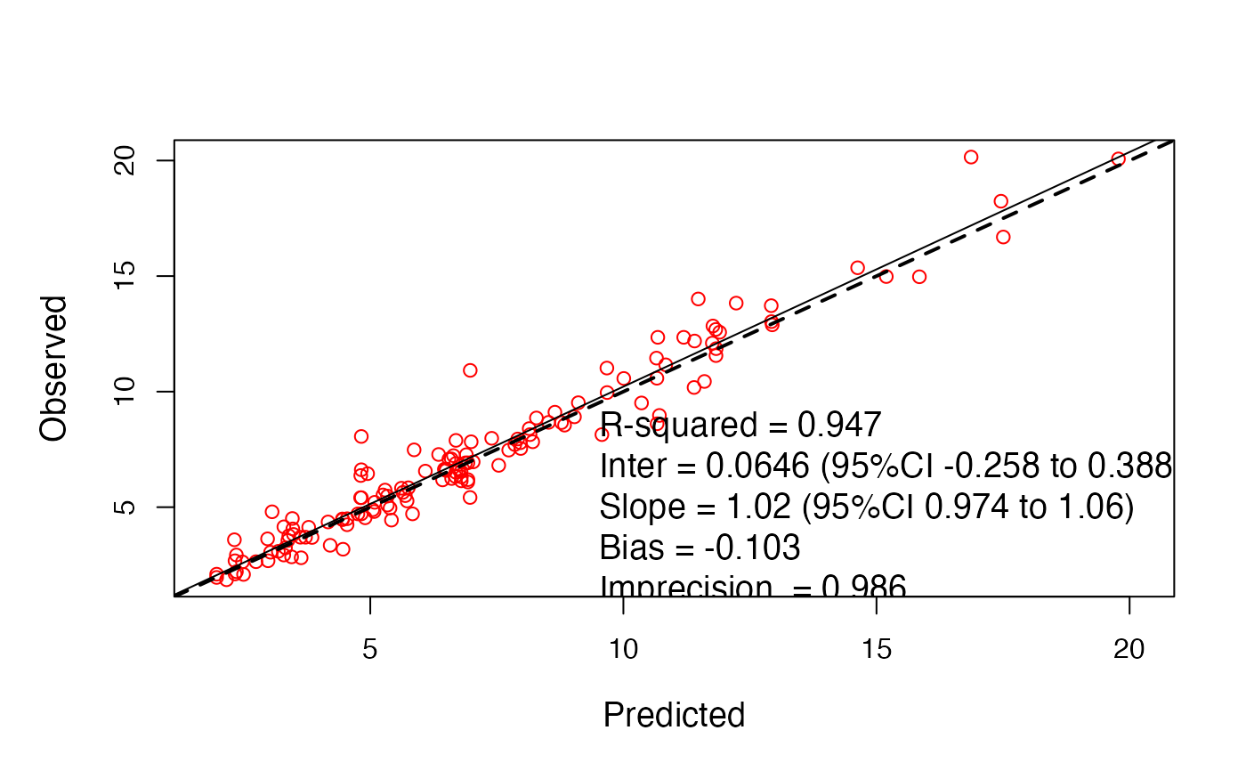
Plot Pmetrics Observed vs. Predicted Objects

It is largely now a legacy plotting function, replaced by plot.PM_op.

Usage

# S3 method for PMop
plot(
  x,
  include,
  exclude,
  pred.type = "post",
  icen = "median",
  outeq = 1,
  mult = 1,
  resid = FALSE,
  log = FALSE,
  square = TRUE,
  ref = TRUE,
  lowess = FALSE,
  reg = TRUE,
  grid,
  ident = FALSE,
  ci = 0.95,
  cex = 1,
  cex.lab = 1.2,
  x.stat = 0.4,
  y.stat = 0.1,
  col.stat = "black",
  cex.stat = 1.2,
  lwd = 2,
  col = "red",
  xlim,
  ylim,
  xlab,
  ylab,
  out = NA,
  ...
)

Arguments

x: The name of an PMop data object generated by makeOP.
include: A vector of subject IDs to include in the plot, e.g. c(1:3,5,15)
exclude: A vector of subject IDs to exclude in the plot, e.g. c(4,6:14,16:20)
pred.type: Either 'post' for a posterior object or 'pop' for a population object. Default is 'post'.
icen: Can be either "median" for the predictions based on medians of pred.type parameter value distributions, or "mean". Default is "median".
outeq: Output equation number. Default is 1.
mult: Multiplication factor for x and y axes, e.g. to convert mg/L to ng/mL. Ignored for residual plots.
resid: Boolean operator to generate a plot of weighted prediction error vs. prediction, a plot of weighted prediction error vs. time, and histogram plot of the weighted prediction errors, with overlying normal distribution of the same mean and variance if ref is true, and a P-value for the Kolmogorov-Smirnov test for non-normality if reg is true. The default is False.
log: Boolean operator to plot in log-log space. This parameter is ignored for residual plots. The default is False
square: Boolean operator to force a observed vs. predicted plots to be square with equal x and y limits. This parameter is ignored for residual plots. The default is True
ref: Boolean operator to draw a reference line of slope 1 in observed vs. predicted plots and slope 0 in residual plots, or a reference normal distribution in residual histogram; the default is True
lowess: Boolean operator to draw a lowess regression line in observed vs. predicted or residual plots; the default is False
reg: Boolean operator to draw a linear regression line and print regression statistics on the plot. For weighted residual plots, it will print the mean weighted prediction error with P value for difference from 0, and the standard deviation of the weighted prediction errors, as well as the probability that the distribution of weighted residuals is not different from normal by the Kolmogorov-Smirnov test. The default is True.
grid: Either a boolean operator to plot a reference grid, or a list with elements x and y, each of which is a vector specifying the native coordinates to plot grid lines; the default is False. For example, grid=list(x=seq(0,24,2),y=1:10). Defaults for missing x or y will be calculated by axTicks. For residual plots, list values for grid will be interpreted as True, i.e. custom grid lines are not allowed.
ident: Boolean operator to plot points as ID numbers; the default is False. This option is useful to identify outliers.
ci: The confidence interval for the linear regression parameter estimates; the default is 0.95.
cex: Size of the plot symbols.
cex.lab: Size of the plot labels.
x.stat: Horizontal position to plot the regression or residual statistics; the units are relative to the origin, i.e. extreme left is 0 and extreme right is 1.
y.stat: Vertical position to plot the regression or residual statistics; the units are relative to the origin, i.e. extreme bottom is 0 and extreme top is 1.
col.stat: Color of the text for the regression or residual statistics.
cex.stat: Size of the text for the regression or residual statistics
lwd: Width of the various regression or reference lines (reference, linear regression, or lowess regression)
col: This parameter will be applied to the plotting symbol and is “red” by default.
xlim: Limits of the x-axis as a vector, e.g. c(0,1). It does not need to be specified, but can be.
ylim: Analogous to xlim
xlab: Label for the x-axis. If missing, will default to “Predicted”.
ylab: Label for the y-axis. If missing, will default to “Observed”.
out: Direct output to a PDF, EPS or image file. Format is a named list whose first argument, type is one of the following character vectors: “pdf”, “eps” (maps to postscript), “png”, “tiff”, “jpeg”, or “bmp”. Other named items in the list are the arguments to each graphic device. PDF and EPS are vector images acceptable to most journals in a very small file size, with scalable (i.e. infinite) resolution. The others are raster images which may be very large files at publication quality dots per inch (DPI), e.g. 800 or 1200. Default value is NA which means the output will go to the current graphic device (usually the monitor). For example, to output an eps file, out=list(“eps”) will generate a 7x7 inch (default) graphic.
...: Other parameters as found in plot.default.

Value

Plots the object.

Details

This function is for PMop objects which can be accessed as the $data object within the $op field of a PM_result object, e.g. PM_result$op$data.

Author

Michael Neely

Examples

library(PmetricsData)
plot(NPex$op$data)