Plot Pmetrics Final Cycle Parameter Value Distributions

Plot objects made by makeFinal. It is largely now a legacy plotting function, replaced by plot.PM_final.

Usage

# S3 method for PMfinal
plot(
  x,
  formula,
  include,
  exclude,
  ref = T,
  cex.lab = 1.2,
  col,
  col.ref,
  alpha.ref = 0.5,
  pch,
  cex,
  lwd,
  lwd.ref,
  density = F,
  scale = 20,
  bg,
  standard = F,
  probs = c(0.05, 0.25, 0.5, 0.75, 0.95),
  legend = T,
  grid = T,
  layout,
  xlab,
  ylab,
  xlim,
  ylim,
  out = NA,
  add = F,
  ...
)

Arguments

x: The name of an PMfinal data object generated by makeFinal
formula: An optional formula of the form y ~ x, where y and x are two model parameters to plot in a 3-dimensional bivariate plot. See details.
include: A vector of subject IDs to include in a Bayesian posterior marginal parameter distribution plot, e.g. c(1:3,5,15). Only relevant for Bayesian posterior plots generated by formula values of the form prob ~ par, where par is a parameter in the model.
exclude: A vector of subject IDs to exclude in a Bayesian posterior marginal parameter distribution plot, e.g. c(4,6:14,16:20). Only relevant for Bayesian posterior plots generated by formula values of the form prob ~ par, where par is a parameter in the model.
ref: Boolean operator to include (if TRUE which is the default) the population marginals in posterior marginal plot as reference.
cex.lab: Size of the plot labels for any univariate or bivariate marginal plot.
col: This parameter will be applied to the histogram lines of a univariate marginal plot, or the central point of a bivariate plot and is "red" by default for the former, and "white" for the latter.
col.ref: Color of reference population marginals included in posterior marginal plots.
alpha.ref: Alpha value for transparency of reference marginals. Default is 0.5, with 0=invisible and 1=opaque.
pch: The plotting character for points in bivariate plots. Default is a cross (pch=3).
cex: The size of the points in bivariate plots
lwd: Width of the histogram lines in the univariate marginal parameter distributions or the thickness of the central points and lines around points in bivariate NPAG plots or around quantiles in the bivariate IT2B plots.
lwd.ref: Width of histogram lines for population marginals included in posterior marginal plots.
density: Boolean operator to plot a kernel density function overlying the histogram of a univarite marginal parameter distribution from NPAG; the default is False. See density. Ignored for IT2B output.
scale: How large to scale the points in a bivariate NPAG plot, relative to their probability. Ignored for IT2B output.
bg: Background fill for points in bivariate NPAG plot. Ignored for IT2B output.
standard: Standardize the normal parameter distribution plots from IT2B to the same scale x-axis. Ignored for NPAG output.
probs: Vector of quantiles to plot on bivariate IT2B plot. Ignored for NPAG plot.
legend: Boolean operator for default if True or list of parameters to be supplied to legend function to plot quantile legend on bivariate IT2B plot. Ignored for NPAG plot.
grid: Boolean operator to plot a grid on either a bivariate NPAG or IT2B plot.
layout: Specify the layout for the plot as c(row,col). Default is as many as needed for all parameters.
xlab: Define x-axis label for bivariate NPAG or IT2B plot. Default is the name of the plotted x-variable.
ylab: Define y-axis label for bivariate NPAG or IT2B plot. Default is the name of the plotted y-variable.
xlim: Limits for the x-axis in a bivariate NPAG or IT2B plot. Default is the range of the x-variable.
ylim: Limits for the y-axis in a bivariate NPAG or IT2B plot. Default is the range of the y-variable.
out: Direct output to a PDF, EPS or image file. Format is a named list whose first argument, type is one of the following character vectors: "pdf", "eps" (maps to postscript), "png], "tiff], "jpeg], or "bmp]. Other named items in the list are the arguments to each graphic device. PDF and EPS are vector images acceptable to most journals in a very small file size, with scalable (i.e. infinite) resolution. The others are raster images which may be very large files at publication quality dots per inch (DPI), e.g. 800 or 1200. Default value is NA which means the output will go to the current graphic device (usually the monitor). For example, to output an eps file, out=list("eps") will generate a 7x7 inch (default) graphic.
add: If TRUE, add plot to existing plot. Default is FALSE.
...: Other parameters as found in plot.default.

Value

Plots the object.

Details

PMfinal objects can be accessed as the $data object within the $final field of a PM_result object, e.g. PM_result$final$data.

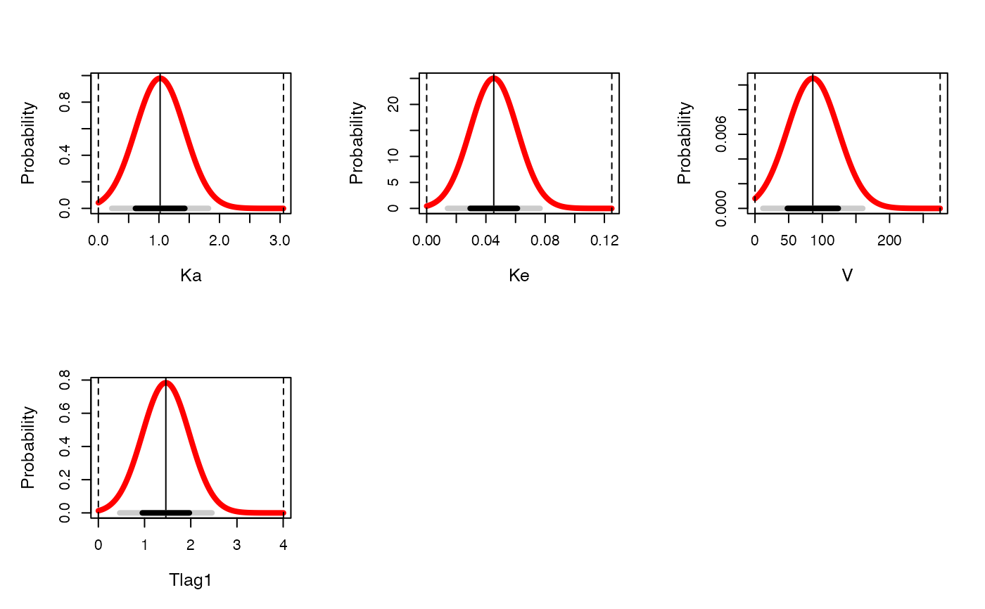
If formula is omitted, this will generate a marginal plot for each parameter. For NPAG data, this will be a histogram of marginal values for each parameter and the associated probability of that value. For IT2B, this will be a series of normal distributions with mean and standard deviation equal to the mean and standard deviation of each parameter marginal distribution, and the standard deviation and 95% distribution indicated at the bottom of each plot. IF formula IS specified, this will generate one of two plots. Specifying "prob" as the y-value vs. a parameter will generate a marginal plot of Bayesian posterior parameter distributions for included/excluded subjects. For example, prob~CL will plot Bayesian posterior distributions for CL for each included/excluded subject.

On the other hand, if formula is two parameters, e.g. CL~V, this will generate a bivariate plot. For NPAG data, it will be support point with size proportional to the probability of each point. For IT2B, it will be an elliptical distribution of a bivariate normal distribution centered at the mean of each plotted variable and surrounding quantiles of the bivariate distribution plotted in decreasing shades of grey.

Author

Michael Neely

Examples

library(PmetricsData)
# NPAG
plot(NPex$final$data)
#> Warning: argument 1 does not name a graphical parameter

# IT2B
plot(ITex$final$data)
#> Warning: argument 1 does not name a graphical parameter