Plot Pmetrics Covariate objects

This method is largely superseded by plot.PM_cov.

Usage

# S3 method for PMcov
plot(
  x,
  formula,
  icen = "median",
  include,
  exclude,
  mult = 1,
  log = F,
  square = F,
  ref = F,
  lowess = F,
  grid = F,
  ident = F,
  reg = F,
  ci = 0.95,
  cex = 1,
  cex.lab = 1.2,
  x.stat = 0.6,
  y.stat = 0.1,
  col.stat = "black",
  cex.stat = 0.8,
  lwd = 2,
  col = "red",
  xlim,
  ylim,
  xlab,
  ylab,
  out = NA,
  ...
)

Arguments

x: The name of an PMcov data object generated by makeCov
formula: This is a mandatory formula of the form y ~ x, where y and x are the two data parameters to plot.
icen: A character vector to summarize covariate and parameter values. Default is “median”, but can also be one of “none”, “mean”. If time is a variable in formula, the value will be set to “none” and the y values will be aggregated by subject ID vs. time.
include: A vector of subject IDs to include in the plot, e.g. c(1:3,5,15)
exclude: A vector of subject IDs to exclude in the plot, e.g. c(4,6:14,16:20)
mult: Multiplication factor for y axis, e.g. to convert mg/L to ng/mL
log: Boolean operator to plot in log-log space; the default is False
square: Boolean operator to force a square plot with equal x and y limits; the default is True
ref: Boolean operator to draw a unity line; the default is True unless “time” is the x value in formula in which case this is ignored
lowess: Boolean operator to draw a lowess regression line; the default is False and this is ignored if “time” is the x value in formula
grid: Either a boolean operator to plot a reference grid, or a list with elements x and y, each of which is a vector specifying the native coordinates to plot grid lines; the default is False. For example, grid=list(x=seq(0,24,2),y=1:10). Defaults for missing x or y will be calculated by axTicks.
ident: Boolean operator to plot points as ID numbers; the default is False. This option is useful to identify outliers.
reg: Boolean operator to draw a linear regression line; the default is True unless “time” is the x value in formula in which case this is ignored. If this option is selected, regression statistics will be printed on the plot if at least 3 subjects are included.
ci: The confidence interval for the linear regression parameter estimates; the default is 0.95.
cex: Size of the plot symbols.
cex.lab: Size of the plot labels.
x.stat: Horizontal position to plot the linear regression statistics; the units are relative to the origin, i.e. extreme left is 0 and extreme right is 1.
y.stat: Vertical position to plot the linear regression statistics; the units are relative to the origin, i.e. extreme bottom is 0 and extreme top is 1.
col.stat: Color of the text for the regression statistics.
cex.stat: Size of the text for the regression statistics.
lwd: Width of the various regression or reference lines (unity, linear regression, or lowess regression)
col: This parameter will be applied to the plotting symbol and is “red” by default.
xlim: Limits of the x-axis as a vector, e.g. c(0,1). It does not need to be specified, but can be.
ylim: Analogous to xlim
xlab: Label for the x-axis. If missing, will default to the name of the x-variable.
ylab: Label for the y-axis. If missing, will default to the name of the y-variable.
out: Direct output to a PDF, EPS or image file. Format is a named list whose first argument, type is one of the following character vectors: “pdf”, “eps” (maps to postscript), “png”, “tiff”, “jpeg”, or “bmp”. Other named items in the list are the arguments to each graphic device. PDF and EPS are vector images acceptable to most journals in a very small file size, with scalable (i.e. infinite) resolution. The others are raster images which may be very large files at publication quality dots per inch (DPI), e.g. 800 or 1200. Default value is NA which means the output will go to the current graphic device (usually the monitor). For example, to output an eps file, out=list(“eps”) will generate a 7x7 inch (default) graphic.
...: Other parameters as found in plot.default.

Value

Plots the object.

Details

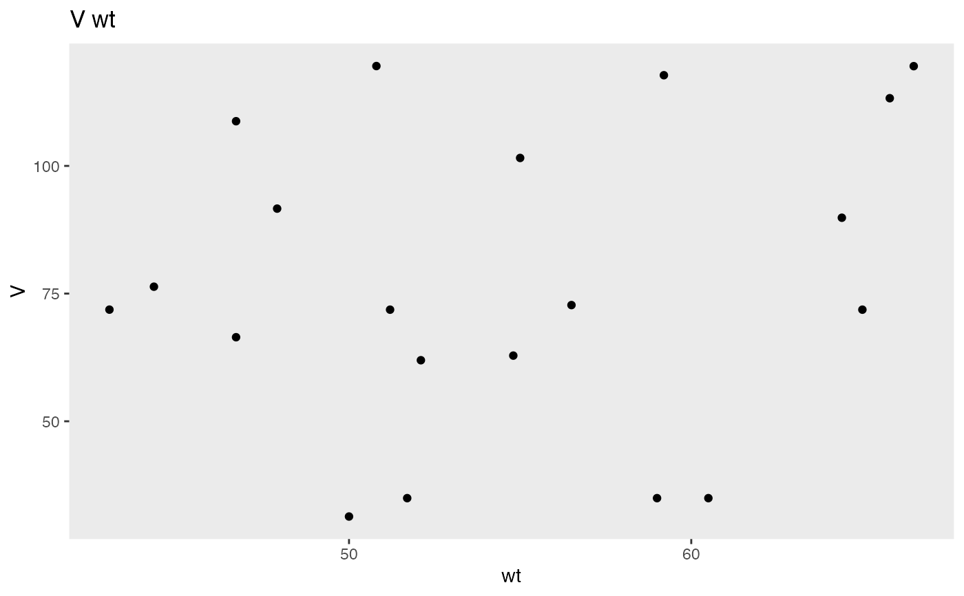
It will plot any two columns, specified using a formula, of a PMcov object, which contains covariate and Bayesian posterior parameter information for each subject. PMcov objects can be accessed as the $data object within the $cov field of a PM_result object, e.g. PM_result$cov$data. Specifying any two variables that do not include time will result in a scatter plot with optional regression and reference lines. If time is included as the x variable, the y variable will be plotted vs. time, aggregated by subject. This can be useful to see time varying parameters, although a formula within formula approach may be required, e.g. plot(cov.1,I(cl_0*wt**0.75)~time) in order to see the change in cl over time according to the change in wt over time, even though cl_0 is constant for a given subject.

Author

Michael Neely

Examples

library(PmetricsData)
plot(NPex$cov$data, V ~ wt)