5  Models

5.1 Introduction

Tip

Make sure you have run the tutorial setup code in your R session before copying, pasting and running example code here.

PM_model objects are one of two fundamental objects in Pmetrics, along with PM_data objects. Defining a PM_model allows for fitting it to the data via the $fit() method to conduct a population analysis, i.e. estimating the probability distribution of model equation parameter values in the population.

5.2 Creating Models

There are three pathways to creating models in Pmetrics.

• Use the new Pmetrics Model Builder app, coming soon. The Shiny app is retired.
• Write a model list in R
• Load an existing model text file

Each of these use sections to define the model. In the app, the sections correspond to tabs. In the list, they are named elements. In the model file, they are code blocks delimited by “#” and the name of the block. The sections are largely the same across the three model pathways, and we’ll cover the details in this document.

5.2.1 Model lists in R

You can write a Pmetrics model list in R. Once in your R script or Quarto document, PM_model list objects can be updated simply by copying, pasting, and editing. This makes it very easy to see how your model evolves during development.

The list elements are the building blocks for the model. Building blocks are of two types.

5.2.1.1 Block types

• Lists define primary parameters, covariates, and error models. These portions of the model are lists of specific creator functions and no additional R code is permissible. Note the commas separating the creator functions, list( to open the list and ) to close the list. Names are case-insensitive and are converted to lowercase for Rust.

# example only; do not execute

# for primary parameters and covariates
block_name = list(     
  var1 = creator(), # var1 is the name of the parameter/covariate   
  var2 = creator(),
  ... # more variables
) # close the list

# for error block
err = list(     
    creator(),   
    creator(),
    ... # as many creators as output equations
) # close the list

• Functions define the other parts of the model, including secondary (global) equations, model equations (e.g. ODEs), lag time, bioavailability, initial conditions, and outputs. These parts of the model are defined as R functions without arguments, but whose body contains any permissible R code. Note the absence of arguments between the (), the opening curly brace { to start the function body and the closing curly brace “}” to end the body. Again, all R code will be converted to lowercase prior to translation into Rust.

# example only; do not execute
block_name = function() { 

      # any valid R code 
      # can use primary or secondary parameters and covariates
      # lines are not separated by commas
      
} # end function and block

Note

All models must have pri, eqn, out, and err blocks.

5.2.2 Model Files

Warning

As of Pmetrics 3.0, you can no longer save models as text files. Model text files should be gradually phased out of your workflow, because it is cumbersome to copy and edit files between runs, and it makes it harder to go back and read the R script to understand how the modeling process evolved unless the script is extensively commented. Having the model code directly in the script is simple to edit and far more transparent. We strongly recommend using model lists in R for all modeling work.

The format of the .txt model file has been mostly unchanged since Pmetrics v.0.4, and such files are created by hand. Once you have a file, it can be loaded in to R with PM_model$new("file"). To facilitate learning the preferred method of defining models directly in R rather than with files, when you create a model from a text file, the R code for the model is copied to the clipboard for easy pasting into your R script or Quarto document.

mod1 <- PM_model$new("src/model.txt") 

The above code will copy the following to your clipbarod, allowing you to paste it into your script or Quarto document.

mod <- PM_model$new(

  pri = list(
    ka = ab(0.100, 0.900),
    ke = ab(0.001, 0.100),
    v = ab(30.000, 120.000),
    lag1 = ab(0.000, 4.000)
  ),
  cov = list(
    wt = interp(),
    africa = interp("none"),
    age = interp(),
    gender = interp("none"),
    height = interp()
  ),
  lag = function () 
  {
      lag[1] = lag1
  },
  eqn = function () 
  {
      two_comp_bolus
  },
  out = function () 
  {
      y[1] = x[2]/v
  },
  err = list(
    proportional(5, c(0.0, 0.1, -0.0, 0.0))
  )

)

Saved models are only text files. You can write files directly yourself, although it is easier and more stable to use the model building app. We will review the format of the files in detail.

Naming your model files. The default model file name is “model.txt,” but you can call them whatever you wish.

Structure of model files. The model file is a text file with up to 9 blocks, each marked by “#” followed by a header tag. For each header, only the capital letters are required for recognition by Pmetrics. The blocks can be in any order, and header names are case-insensitive (i.e. the capitalization here is just to show which letters are required). We include a complete examples.

You can insert comments into your model text file by starting a line with a capital “C” followed by a space. These lines will be removed/ignored in the final Rust code.

5.3 Model Blocks

Blocks common to all the model building pathways include the following. The capital letters are the shorthand way to designate the blocks in the R list format or model text files.

• PRImary variables
• COVariates
• SECcondary variables
• INItial conditions
• FA (bioavailability)
• LAG time
• EQuatioNs
• OUTputs
• ERRors

5.3.1 Model Library

You can access the Pmetrics Model Library programmatically using the model_lib function. This function returns a data frame of available models with their characteristics, including the model name to be used in the EQN block, number of compartments, number of inputs and outputs, and a brief description.

All of the models are pre-loaded as R6 objects. You can get details of the model by simply typing its primary name from the table into the console. For example:

# see the library contents
model_lib()
# an example of a model in the library
two_comp_bolus

5.3.2 PRImary

5.3.2.1 List

Primary variables are defined in a list(). The list is named “pri”, and is comprised of named elements which are the parameters, and the creator function to define each parameter, one parameter to a line.

The two creator functions for primary parameters are ab and msd. Choose one for each parameter. The first defines the absolute search space for that parameter for NPAG/NPOD, i.e., the range. msd is the companion function that specifies the range using a mean and standard deviation (SD), assuming the mean is the midpoint of the range, and the SD equals 1/6th of the range, i.3., there are 3 SD above and below the mean, covering 99.7% of the prior distribution.

# this is only a partial model snippet for illustration; do not execute
mod <- PM_model$new(
  pri = list(
    Ke = ab(0, 5), # mean will be 2.5, SD = 5/6 = 0.83
    V = msd(100, 20) # range will be 100 ± 3*20, i.e. [40, 160]
  )
)

5.3.2.2 File

Primary variables are a list of variable names, one name to a line. On each line, following the variable name, is the range for the parameter that defines the search space. These ranges behave slightly differently for NPAG and the simulator.

• For all engines, the format of the limits is min, max.

• For NPAG/NPOD, when min, max limits are specified, they are absolute, i.e. the algorithm will not search outside this range.

• The simulator will ignore the ranges with the default value of NULL for the limits argument to PM_sim. If the simulator limits argument is set to NA, it will mean that these ranges will be used as the limits to truncate the simulation.

Example:

#Pri
KE, 0, 5
V, 0.01, 100
KA, 0, 5

5.3.3 COVariates

Covariates are subject-specific data, such as body weight, contained in the data. The covariate names, which are the column names in the data file or PM_data object, must be declared if used in the model object. Once declared, they can be used in secondary variable and differential equations. The names should be the same as in the data file.

By default, missing covariate values are linearly interpolated between existing values, or carried forward if the first value is the only non-missing entry. However, you can suppress interpolation and carry forward the previous value in a piece-wise constant fashion, depending on the way you define the model as described below.

5.3.3.1 List

The covariate element is a list whose names are the same as the covariates in the data file, and whose values are the interp creator function to declare how each covariate is interpolated between entries in the data.

The default argument for interp is “lm” which means that values will be linearly interpolated between entries, like the R linear model function lm. The alternative is “none”, which holds the covariate value the same as the previous entry until it changes, i.e., a carry-forward strategy.

# this is only a partial model snippet for illustration; do not execute
mod <- PM_model$new(
  pri = list(...),
  cov = list(
      wt = interp(),
      age = interp("none")
    )
)

Here, wt will be linearly interpolated and age will be piece-wise constant, i.e. held constant until the next entry in the data file.

5.3.3.2 File

List the covariates by name, one per line in the #COV block. To make a covariate piece-wise constant, include an exclamation point (!) in the declaration line.

Note that any covariate relationship to any parameter may be described as the user wishes by mathematical equations and R code, allowing for exploration of complex, non-linear, time-dependent, and/or conditional relationships. These equations are included in any of the blocks which are functions (SEC, EQN, INI, FA, LAG, OUT).

Example:

#Cov
wt
cyp
IC!

Here, IC will be piece-wise constant and the other two will be linearly interpolated for missing values.

5.3.4 Secondary

Secondary variables are those that are defined by equations that are combinations of primary, covariates, and other secondary variables. Pmetrics does NOT generate distributions for the values of secondary variables. They are only used internally to define the model. Variables declared in the secondary block are global, i.e., they are available to all other blocks. This is in contrast to variables declared within other function blocks (INI, FA, LAG, OUT), which are only available within the block they are declared.

5.3.4.1 List

Specify each variable equation as a list of unnamed character elements in the same way as for the app. In the example below, V0 is the primary parameter which will be estimated, but internally, the model uses V as V0*wt, unless age is >18, in which case weight is capped at 75 kg. It’s the same for CL0. Note that the conditional statement is not named.

# this is only a partial model snippet for illustration; do not execute
mod <- PM_model$new(
    pri = list(
      CL0 = ab(0, 5),
      V0 = msd(10, 3)
    ),
    cov = list(
      wt = interp(),
      age = interp()
    ),
    sec = function(){
      V = V0*wt
      if (age >18) {V = V0 * 75}
      CL = CL0 * wt
    }
) # end of $new()

5.3.4.2 File

Format is the same as for equations in the list.

Example:

#Sec
CL = Ke * V * wt**0.75
if (cyp > 1) {CL = CL * cyp}

5.3.5 INItial conditions

By default, all model compartments have zero amounts at time 0. However, you can change the default initial condition of any compartment from 0 to something else. It can be an fixed value, primary or secondary variables, or covariate(s), or equations/conditionals based on these.

5.3.5.1 List

Initial conditions can be changed as a function called “ini”. Each line of the function specifies the compartment amount as “X[.] = expression”, where “.” is the compartment number. Primary and secondary variables and covariates may be used in the expression, as can conditional statements in R syntax.

# this is only a partial model snippet for illustration; do not execute 
mod <- PM_model$new(
    pri = list(
      Ke = ab(0, 5),
      V = msd(100, 30),
      IC3 = ab(0, 1000)
    ),
    cov = list(
      wt = interp(),
      age = interp(),
      IC2 = interp("none")
    ),
    ini = function(){
      X[1] = IC2*V
      X[3] = IC3
    }
) # end of $new()

In the example above, IC2 is a covariate with the measured trough concentration prior to an observed dose and IC3 is a fitted primary parameter specifying an initial amount in unobserved compartment 3.

In the first case, the initial condition for compartment 2 becomes the value of the IC2 covariate (defined in cov list) multiplied by the current estimate of V during each iteration. This is useful when a subject has been taking a drug as an outpatient, and comes in to the lab for PK sampling, with measurement of a concentration immediately prior to a witnessed dose, which is in turn followed by more sampling. In this case, IC2 or any other covariate can be set to the initial measured concentration, and if V is the volume of compartment 2, the initial condition (amount) in compartment 2 will now be set to the measured concentration of drug multiplied by the estimated volume for each iteration until convergence.

In the second case, the initial condition for compartment 3 becomes another variable, IC3 defined in the pri list, to fit in the model, given the observed data.

5.3.5.2 File

The same example as for the list above is shown below in the format for the file.

#Ini
X[2] = IC*V
X[3] = IC3

5.3.6 FA (bioavailability)

In this tab you can change the default bioavailability of any bolus input from 1 to something else. It can be an equation, primary or secondary variable, or covariate.

5.3.6.1 List

Bioavailability for any bolus input can be changed from the default value of 1. Use a function called “fa”, where each line is of the form “FA[.] = expression”, and “.” is the input number. Primary and secondary variables and covariates may be used in the expression, as can conditional statements.

# this is only a partial model snippet for illustration; do not execute
mod <- PM_model$new(
    pri = list(
      Ke = ab(0, 5),
      V = msd(100, 30),
      FA1 = ab(0, 1)
    ),
    fa = function(){
      FA[1] = FA1
    }
)

5.3.6.2 File

The same example as for the list above is shown below in the format for the file.

#Fa
FA[1] = FA1

5.3.7 LAG time

The lag time is a delay in absorption for a bolus input.

5.3.7.1 List

Use a function called “lag”, each line of the form “LAG[.] = expression”, where “.” is the input number. Primary and secondary variables and covariates may be used in the expression, as can conditional statements.

# this is only a partial model snippet for illustration; do not execute 
mod <- PM_model$new(
    pri = list(
      Ke = ab(0, 5),
      V = msd(100, 30),
      lag1 = ab(0, 4)
    ),
    lag = function(){
      LAG[1] = lag1
    }
)

5.3.7.2 File

The same example as for the list above is shown below in the format for the file.

#Lag
LAG[1] = Tlag1

5.3.8 EQuatioNs

These are the equations that define the structural model, i.e., the mathematical expressions that relate input (dose) to output (measurements). Pmetrics has a library of models with algebraic solutions and models can also use differential equations in a format compatible with R. Even algebraic models will contain differential equations for purposes of understanding and plotting the model, but algebraic models from the library include a token which tells Pmetrics how to choose the correct model. Details below.

5.3.8.1 List

Specify a model as a function called “eqn”, with each element an ordinary differential equation in R syntax. Additional equations can be included. Special elements are as follows:

• dX[.] is the change in amount in compartment “.”, e.g. dX[1] for compartment 1. This is shorthand for \(dX/dt\).
• X[.] is the amount in compartment “.”, e.g. X[2] for compartment 2.
• B[.] or BOLUS[.] is the bolus input number “.”, e.g. B[1] for bolus input 1. Note the the number is not the compartment number, but the number of the input, corresponding to the INPUT column in the data file. Which compartment the bolus enters is defined by which equation includes B[.].
• R[.] or RATEIV[.] is the infusion input number “.”, e.g. R[1] for infusion input 1, again corresponding to the data INPUT number, not the compartment number.

If your data file has dose inputs with DUR = 0, these are considered to be instantaneous bolus inputs, and you must use B[.] or BOLUS[.] to represent them in the equations. If your data file has dose inputs with DUR > 0, these are considered to be infusions, and you should use R[.] or RATEIV[.] to represent them in the equations.

Tip

Local variables defined within the eqn function are not available outside the function. If you wish to use a variable in other blocks, define it in the sec function to make it global.

# this is only a partial model snippet for illustration; do not execute 
mod <- PM_model$new(
    pri = list(
      Ka = ab(0, 5),
      Ke = ab(0, 5),
      V = msd(100, 30),
      Kcp = ab(0, 5),
      Kpc = ab(0, 5)
    ),
    eqn = function(){
      ktotal = Ke + Kcp # local variable, not available outside eqn block
      dX[1] = B[1] - Ka * X[1]
      dX[2] = R[1] + Ka * X[1] - (ktotal) * X[2] + Kpc * X[3]
      dX[3] = Kcp * X[2] - Kpc * X[3]
    }
)

To specify models from the library, first ensure the correct library model name by using the model_lib function. Also, ensure that the variable names in the library are defined somewhere in the model (mostly in the PRI block), and similarly that OUT equations are correct.

# this is a full example of a model that can be compiled
mod <- PM_model$new(
    pri = list( # parameter names match those listed in model_lib(), except V0
      Ka = ab(0, 5),
      Ke = ab(0, 5),
      V0 = msd(10, 3),
      Kcp = ab(0, 5),
      Kpc = ab(0, 5)
    ),
    cov = list(
        wt = interp()
    ),
    sec = function(){
        V = V0 * wt # here we define the last parameter, V, found in model_lib() for this model
    },
    eqn = function(){
        "three_comp_bolus" # name acquired from model_lib()
    }, 
    out = function(){
        Y[1] = X[2]/V # correct compartment (2) identified as the output
    },
    err = list(
        proportional(1, c(1, 0.1, 0, 0))
    )
)

5.3.8.2 File

Use the same syntax as in the R function in a list specification.

Example:

#EQN
ktotal = Ke + KCP
dX[1] = B[1] -KA*X[1]
dX[2] = R[1] + KA*X[1] - (ktotal)*X[2] + KPC*X[3]
dX[3] = KCP*X[2] - KPC*X[3]

Note: Pmetrics no longer recognizes the old Fortran format of XP(1), which is dX[1], and X(1), which is X[1].

5.3.9 Outputs

The outputs in Pmetrics are the values in the OUT column of the data that you are trying to predict. In the model objects, each output is referred to as Y[.], where “.” is the number of the output and the same as the corresponding OUTEQ in the data. Outputs can be defined as mathematical combinations of compartment amounts (X[.]), primary and/or secondary parameters, or covariates.

Output equations are in R format. If they include conditional statements, these should follow R’s if(){} convention.

5.3.9.1 List

The out element of the model list is function. Any R code is valid within the function. Secondary variables declared here will only be available within the function. The output equations are of the form “Y[.] = expression”, where “.” is the output equation number in the data. Primary and secondary variables and covariates may be used in the expression, as can conditional statements in R code.

# this is only a partial model snippet for illustration; do not execute
out = function(){
  Y[1] = X[1]/V
}

5.3.9.2 File

Outputs are of the form Y[.] = expression, where “.” is the output equation number. Primary and secondary variables and covariates may be used in the expression, as can conditional statements in Fortran code. An “&” continuation prefix is not necessary in this block for any statement, although if present, will be ignored. There can be a maximum of 6 outputs. They are referred to as Y[1], Y[2], etc. These equations may also define a model explicitly as a function of primary and secondary variables and covariates.

Examples:

#Out
Y[1] = X[2]/V

Here’s an example of an explicit model defined in the output and not the equation block.

#OUT

RES = BOLUS[1] * KIN/(KIN-KOUT) * (EXP(-KOUT*TPD)-EXP(-KIN*TPD))
Y[1] = RES/VD

5.3.10 Error

All models predict observations with error. Part of this error is due to measurement or assay error. The assay error in Pmetrics is explicitly accounted for, and it may be inflated by an additive model error component \(\lambda\) or a proportional component \(\gamma\) that reflect additional noise and model misspecification. The remaining error is random and not optimized.

When fitting, the error in a prediction determines how closely the model must match the observation. Pmetrics weights predictions by \(1/error^2\). The standard deviation of an prediction is calculated from the assay error model as \(SD_{pred} = C0 + C1*pred + C2*pred^2 + C3*pred^3\). Error is then calculated according to the selected model error structure:

• Proportional: \(error = \gamma * SD_{pred}\)
• Additive: \(error = \lambda + SD_{pred}\)

Note: Each output equation must have an error model. In Pmetrics versions prior to 3.0.0, each output equation had its own assay error polynomial, but there was only one model error for all outputs. In Pmetrics ≥ 3.0.0, each output equation has its own assay error polynomial and its own model error, allowing for greater flexibility in modeling complex data.

5.3.10.1 List

The error list element is a list of creator functions. The two possible creator functions are proportional or additive. Each of these functions has the same arguments: initial, coeff, and fixed.

• The initial argument is the starting value for \(\gamma\) in the proportional() creator function or \(\lambda\) for the additive() creator function.
• For both creators, coeff is the vector of 4 numbers that defines a polynomial equation to permit calculation of the standard deviation of an observation, based on the noise of the assay (see makeErrorPoly).
• The final argument fixed is FALSE by default, which means that \(\gamma\) or \(\lambda\) will be estimated for each output equation as measures of additional noise in the data and/or model misspecification. If fixed is set to TRUE, then the value in initial will be held constant during estimation.

In the code snippet below, there are two output equations so there are two error models. The first is a \(\gamma\) proportional model with starting value 1, which will be updated based on the model fit of the data, and assay polynomial coefficients of 0.15, 0.1, 0, and 0. The second is an additive \(\lambda\) model with starting value 0.1, assay polynomial coefficients of 0.1, 0, 0, and 0, and because fixed = TRUE, it will not be estimated and will be held constant at 0.1.

# this is only a partial model snippet for illustration; do not execute
mod <- PM_model$new(
  out = function(){
    Y[1] = X[1]/V1
    Y[2] = X[2]/V2
  },
  err = list(
    proportional(1, c(0.15, 0.1, 0, 0)),
    additive(0.1, c(0.1, 0, 0, 0), fixed = TRUE)
  )
)

5.3.10.2 File

Unlike the R6 model builder app or model list, the error block in the file is separated from the output block. This is to maintain backward compatibility with Legacy Pmetrics.

To specify the model in this block, each output requires two lines. The first line is either L=number or G=number for a \(\lambda\) or \(\gamma\) error model. The number is the starting value for \(\lambda\) or \(\gamma\). If you include an exclamation point (!) in the declaration, then \(\lambda\) or \(\gamma\) will be fixed and not estimated.

The second line contains the values for the assay error polynomial coefficients: \(C0\), \(C1\), \(C2\), and \(C3\), separated by commas. Pmetrics will use these values for the coefficients unless they are included in the data.

Example 1: estimated \(\lambda\), starting at 0.4, one output, use 0.1,0.1,0,0 for the coefficients unless present in the data.

#Err
L=0.4
0.1,0.1,0,0

Example 2: two outputs with fixed \(\gamma\) of 2 for output 1, and \(\lambda\) with starting value of 0.1 but estimated for output 2. Coefficients of 0.1,0.1,0,0 for the first output, and 0.3, 0.1, 0, 0 for output 2.

#Err
G=2!
0.1,0.1,0,0
L=0.1
0.3,0.1,0,0

5.4 Complete Model Examples

5.4.1 List Examples

Here are two complete examples of model definitions using the list format.

# this example of a one-compartment IV model will compile 
mod1 <- PM_model$new(
  pri = list(
    Ke = ab(0, 5),
    V = msd(100, 30)
  ),
  eqn = function(){
    one_comp_iv # in model_lib()
  },
  out = function(){
    Y[1] = X[1]/V
  },
  err = list(
    proportional(5, c(0.05, 0.1, 0, 0))
  )
)

ℹ Compiling model...

Using template path: /Library/Frameworks/R.framework/Versions/4.5-arm64/Resources/library/Pmetrics 

When you execute the above code in your own script or Quarto document, you will see a message indicating that the model has compiled.

Notes:

• The #Pri block contains the primary parameters and their initial ranges, which are the only parameters that will be estimated.
  • Ke is the elimination rate constant defined by the creator function ab() with lower and upper bounds of 0 and 5, respectively.
  • V is the volume of distribution defined by the creator function msd() with a
• The value of “one_comp_iv” in the #Eqn block tells Pmetrics to use the algebraic solution for the model in the library.
• The #Out block contains the output equation. The relevant compartment number that contains the amount of drug, 1, is obtained by looking at model_lib() to see which compartment is the central, so that it can be divided by V to obtain concentration.
• The #Err block contains the model error structure (proportional) with a starting \(\gamma\) value of 5, and assay error coefficients of 0.05, 0.1, 0, and 0.
• The comments in the code above will be ignored.

You can see a summary of the model by printing the model object, and you can plot the model structure by calling the plot() method.

mod1 # prints the model object

── Model summary ───────────────────────────────────────────────────────────────

── Primary Parameters 

Ke: [0, 5], ~N(2.5, 0.83)

V: [10, 190], ~N(100, 30)

── Covariates 

── Primary Equations 

one_comp_iv

── Outputs 

Y[1] = X[1]/V

── Error Model 

Proportional, with initial value of 5 and coefficients 0.05, 0.1, 0, and 0.

mod1$plot() #plots the model structure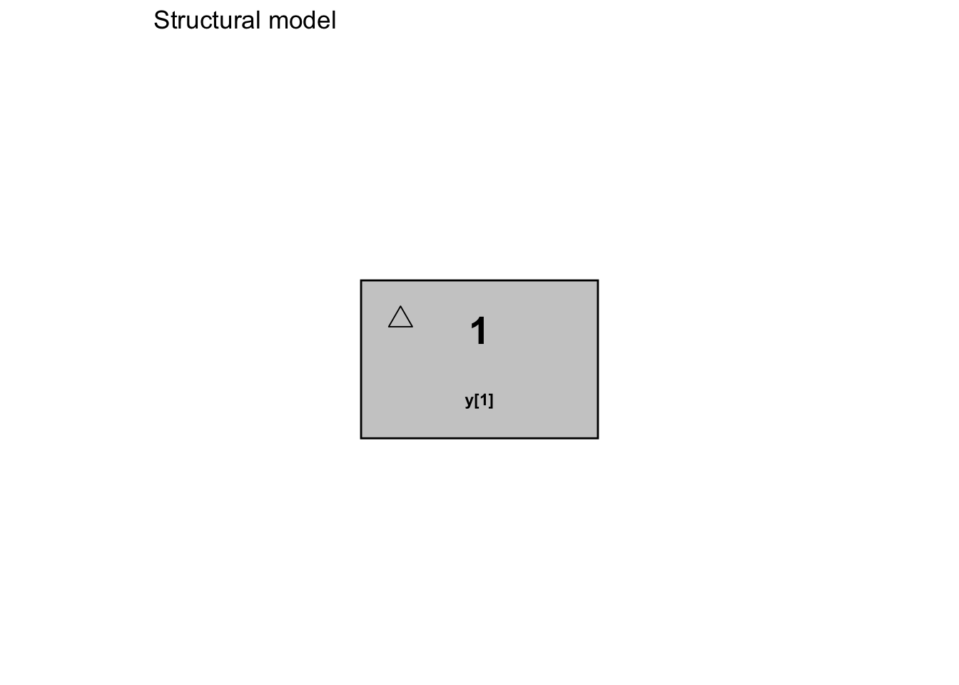

Here’s an example for a parent and metabolite showing differential equations and multiple outputs .

# this example of a parent and metabolite model will compile
mod2_ode <- PM_model$new(
  pri = list(
    Ka = ab(0, 5),
    Ke = ab(0, 5),
    V = msd(100, 30),
    fm = ab(0, 1),
    Ke_m = ab(0, 5)
  ),
  eqn = function(){
    # same as two_comp_bolus in model_lib()
    dX[1] = B[1] - Ka * X[1] # bolus input here with B[1]
    dX[2] = R[1] + Ka * X[1] - Ke * X[2] # can also accept infusion input here with R[1]
    dX[3] = fm * X[2] - Ke_m * X[3] # a metabolite compartment
  },
  out = function(){
    Vm = V * 0.5 # fix metabolite volume at 50% of parent
    Y[1] = X[1]/V
    Y[2] = X[3]/Vm
  },
  err = list( # one error model for each output
    proportional(5, c(0.05, 0.1, 0, 0)),
    additive(0.1, c(0.1, 0, 0, 0))
  )
)

5.4.2 File Example

Here is a complete example of a model file, as of Pmetrics version 3.0 and higher:

#Pri
KE, 0, 5
V0, 0.1, 100
KA, 0, 5
Lag1, 0, 3

#Cov
wt
C this weight is in kg

#Sec
V = V0*wt

#Lag
LAG[1] = Tlag1

#Eqn
two_comp_bolus

#Out
Y[1] = X[2]/V

#Err
L=0.4
0.1, 0.1, 0, 0

Notes:

• The #Pri block contains the primary parameters and their initial ranges, which are the only parameters that will be estimated.
• The #Cov block contains the covariate names.
• The #Sec block contains the global secondary equations used to incorporate the covariate “wt” in the model definition.
• The #Lag block contains the lag time for the bolus input.
• The value of “two_comp_bolus” in the #Eqn block tells Pmetrics to use the algebraic solution for the model.
• The #Out block contains the output equation. The relevant compartment number that contains the amount of drug, 2, is obtained by looking at model_lib() to see which compartment is the central, so that it can be divided by V to obtain concentration.
• The #Err block contains the model error structure (additive) with a starting \(\lambda\) value of 0.4, and assay error coefficients of 0.1, 0.1, 0, and 0.
• The comment line “C this weight is in kg” will be ignored.

Create and save such a file in any text editor, giving it a name ending in “.txt”.

PM_model$new() also accepts the path to a model file to create the same model using the file. Remember that you should phase model files out of your workflow in favor of direct definition in R.

ℹ Compiling model...

Using template path: /Library/Frameworks/R.framework/Versions/4.5-arm64/Resources/library/Pmetrics 

── Model summary ───────────────────────────────────────────────────────────────

── Primary Parameters 
ka: [0.1, 0.9], ~N(0.5, 0.13)
ke: [0.001, 0.1], ~N(0.05, 0.02)
v: [30, 120], ~N(75, 15)
lag1: [0, 4], ~N(2, 0.67)

── Covariates 
wt, africa (no interpolation), age, gender (no interpolation), and height

── Primary Equations 
two_comp_bolus

── Lag Time 
lag[1] = lag1

── Outputs 
y[1] = x[2]/v

── Error Model 
Proportional, with initial value of 5 and coefficients 0.02, 0.05, -2e-04, and
0.

# if not using the Rscript/Learn.R template created by PM_tutorial(), 
# modify the path as needed
mod1b <- PM_model$new("src/model.txt")
mod1b # look at it

5.5 Reserved Names

The following cannot be used as primary, covariate, or secondary variable names. They can be used in equations, however.

Reserved.Variable	Function.in.Pmetrics
t	time
x	array of compartment amounts
dx	array of first derivative of compartment amounts
p	array of primary parameters
rateiv / r	infusion vector
bolus / b	bolus vector
cov	covariate hashmap
y	output vector

5.6 Updating models

5.6.1 List

To update a model, simply copy the text from the model list in R, and modify the relevant fields. Then reassign the modified model to a new object.

# these examples will compile and can be executed 

mod1 <- PM_model$new(
  pri = list(
    Ka = ab(0.1, 0.9),
    Ke = ab(0.001, 0.1),
    V = ab(30, 120),
    lag1 = ab(0, 4)
  ),
  cov = list(
    wt = interp(),
    africa = interp("none"),
    age = interp(),
    gender = interp("none"),
    height = interp()
  ),
  eqn = function() {
    two_comp_bolus
  },
  lag = function() {
    lag[1] <- lag1
  },
  out = function() {
    Y[1] <- X[2] / V
  },
  err = list(
    proportional(5, c(0.02, 0.05, -0.0002, 0))
  )
)

mod2 <- PM_model$new(
  pri = list(
    Ka = ab(0.1, 0.9),
    Ke = ab(0.001, 0.5), # changed range
    V0 = ab(30, 120), # note the new name
    lag1 = ab(0, 4)
  ),
  cov = list(
    wt = interp(),
    africa = interp("none"),
    age = interp(),
    gender = interp("none"),
    height = interp()
  ),
  sec = function() { # new secondary block
    V = V0 * wt # the library model expects a parameter named "V" defined somewhere
  },
  eqn = function() {
    two_comp_bolus
  },
  lag = function() {
    lag[1] <- lag1
  },
  out = function() {
    Y[1] <- X[2] / V
  },
  err = list(
    proportional(5, c(0.02, 0.05, -0.0002, 0))
  )
)

This example changes the range of Ke, deletes V, adds V0, and defines a new secondary relationship for V = V0 * wt.

5.6.2 File

The only way to update a model file is to edit the text file and load it with PM_model$new(). The disadvantage is that you have to keep editing, copying and pasting files, and unless your documentation in R or elsewhere is good, you have no idea how you changed the model from run to run. In contrast, by using the direct model definition in R, you can see a written record in your script of how the model evolved over the project.